Quantum Bayesian Network Sampling (pyagrum.qBNSampling)
|
|
|
|
|





The pyagrum.qBNSampling module encodes a Bayesian network as a quantum circuit so that measuring the circuit samples from the network’s joint distribution. It also provides a quantum rejection-sampling inference engine that computes posterior distributions conditioned on evidence using Grover-based amplitude amplification.
Dependencies: qiskit, qiskit-aer, qiskit-ibm-runtime, scipy.
References
Circuit encoding: Borujeni et al., Quantum circuit representation of Bayesian networks, Expert Systems with Applications, 2021. arXiv:2004.14803
Quantum inference: Low, Yoder, Chuang, Quantum inference on Bayesian networks, Physical Review A, 2014. arXiv:1402.7359
In [1]:
import pyagrum as gum
import pyagrum.lib.notebook as gnb
import pyagrum.qBNSampling as qBNS
Part 1 — qBNMC: encoding a Bayesian network as a quantum circuit
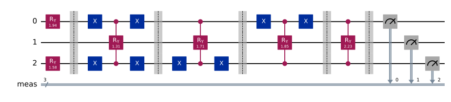
Each variable in the BN is mapped to \(\lceil \log_2(|\text{dom}|) \rceil\) qubits. Its CPT is encoded as multi-qubit RY rotations: root nodes get unconditional rotations; non-root nodes get controlled rotations — one block per parent configuration, framed by X gates to select the correct control state.
Measuring the circuit returns a sample from the joint distribution of the network.
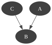
Illustrative example: 3-node BN
In [2]:
bn = gum.fastBN("A->B<-C", 2)
gnb.showBN(bn)
In [3]:
qbn = qBNS.qBNMC(bn)

print(f"Total qubits: {qbn.getTotNumQBits()}")
print(f"Qubit map (node id -> qubit ids): {qbn.n_qb_map}")

circuit = qbn.buildCircuit(add_measure=True)
Total qubits: 3
Qubit map (node id -> qubit ids): {0: [0], 1: [1], 2: [2]}
Running the circuit on the Aer simulator returns marginal probability vectors for each variable. Let us compare them with the exact marginals from LazyPropagation.
In [4]:
gnb.showBN(bn)
In [5]:
circuit.draw("mpl", scale=0.7) # nbsphinx-thumbnail
Out[5]:
In [6]:
circuit.draw("latex")
Out[6]:

In [7]:
circuit.draw()
Out[7]:
        ┌────────────┐ ░ ┌───┐              ┌───┐ ░                          ░ »
     0: ┤ Ry(1.9356) ├─░─┤ X ├──────■───────┤ X ├─░────────────■─────────────░─»
        └────────────┘ ░ └───┘┌─────┴──────┐└───┘ ░      ┌─────┴──────┐      ░ »
     1: ───────────────░──────┤ Ry(1.3092) ├──────░──────┤ Ry(1.7069) ├──────░─»
        ┌────────────┐ ░ ┌───┐└─────┬──────┘┌───┐ ░ ┌───┐└─────┬──────┘┌───┐ ░ »
     2: ┤ Ry(1.5829) ├─░─┤ X ├──────■───────┤ X ├─░─┤ X ├──────■───────┤ X ├─░─»
        └────────────┘ ░ └───┘              └───┘ ░ └───┘              └───┘ ░ »
meas: 3/═══════════════════════════════════════════════════════════════════════»
                                                                               »
«        ┌───┐              ┌───┐ ░                ░ ┌─┐
«     0: ┤ X ├──────■───────┤ X ├─░───────■────────░─┤M├──────
«        └───┘┌─────┴──────┐└───┘ ░ ┌─────┴──────┐ ░ └╥┘┌─┐
«     1: ─────┤ Ry(1.8542) ├──────░─┤ Ry(2.2282) ├─░──╫─┤M├───
«             └─────┬──────┘      ░ └─────┬──────┘ ░  ║ └╥┘┌─┐
«     2: ───────────■─────────────░───────■────────░──╫──╫─┤M├
«                                 ░                ░  ║  ║ └╥┘
«meas: 3/═════════════════════════════════════════════╩══╩══╩═
«                                                     0  1  2
In [8]:
marginals = qbn.runBN(shots=10000)
In [9]:
ie = gum.LazyPropagation(bn)
ie.makeInference()

for name, tensor in marginals.items():
  print(f"P({name})")
  print(f"  qBNMC (10 000 shots) : {[round(v, 4) for v in tensor.tolist()]}")
  print(f"  LazyPropagation      : {[round(v, 4) for v in ie.posterior(name).tolist()]}")
  print()
P(A)
  qBNMC (10 000 shots) : [0.3226, 0.6774]
  LazyPropagation      : [0.3216, 0.6784]

P(B)
  qBNMC (10 000 shots) : [0.3721, 0.6279]
  LazyPropagation      : [0.3701, 0.6299]

P(C)
  qBNMC (10 000 shots) : [0.4861, 0.5139]
  LazyPropagation      : [0.4939, 0.5061]
Named example: Oil Company Stock Price (Borujeni et al., 2021)
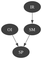
A 4-node BN modelling the dependencies between Interest Rate (IR), Stock Market (SM), Oil Import (OI), and Stock Price (SP).
In [10]:
bn_oil = gum.fastBN("IR->SM->SP<-OI", 2)
bn_oil.cpt("IR")[:] = [0.75, 0.25]
bn_oil.cpt("SM")[:] = [[0.3, 0.7], [0.8, 0.2]]
bn_oil.cpt("OI")[:] = [0.6, 0.4]
bn_oil.cpt("SP")[:] = [[[0.1, 0.9], [0.3, 0.7]], [[0.4, 0.6], [0.7, 0.3]]]

gnb.showBN(bn_oil)
In [11]:
qbn_oil = qBNS.qBNMC(bn_oil)
print(f"Total qubits: {qbn_oil.getTotNumQBits()}")
qbn_oil.buildCircuit().draw("text")
Total qubits: 4
Out[11]:
         ┌─────────┐   ░ ┌───┐              ┌───┐ ░                ░      »
     0: ─┤ Ry(π/3) ├───░─┤ X ├──────■───────┤ X ├─░───────■────────░──────»
         └─────────┘   ░ └───┘┌─────┴──────┐└───┘ ░ ┌─────┴──────┐ ░ ┌───┐»
     1: ───────────────░──────┤ Ry(1.9823) ├──────░─┤ Ry(0.9273) ├─░─┤ X ├»
                       ░      └────────────┘      ░ └────────────┘ ░ └───┘»
     2: ───────────────░──────────────────────────░────────────────░──────»
        ┌────────────┐ ░                          ░                ░ ┌───┐»
     3: ┤ Ry(1.3694) ├─░──────────────────────────░────────────────░─┤ X ├»
        └────────────┘ ░                          ░                ░ └───┘»
meas: 4/══════════════════════════════════════════════════════════════════»
                                                                          »
«                            ░                          ░                    »
«     0: ────────────────────░──────────────────────────░────────────────────»
«                      ┌───┐ ░                          ░ ┌───┐              »
«     1: ──────■───────┤ X ├─░────────────■─────────────░─┤ X ├──────■───────»
«        ┌─────┴──────┐└───┘ ░      ┌─────┴──────┐      ░ └───┘┌─────┴──────┐»
«     2: ┤ Ry(2.4981) ├──────░──────┤ Ry(1.9823) ├──────░──────┤ Ry(1.7722) ├»
«        └─────┬──────┘┌───┐ ░ ┌───┐└─────┬──────┘┌───┐ ░      └─────┬──────┘»
«     3: ──────■───────┤ X ├─░─┤ X ├──────■───────┤ X ├─░────────────■───────»
«                      └───┘ ░ └───┘              └───┘ ░                    »
«meas: 4/════════════════════════════════════════════════════════════════════»
«                                                                            »
«              ░                ░ ┌─┐
«     0: ──────░────────────────░─┤M├─────────
«        ┌───┐ ░                ░ └╥┘┌─┐
«     1: ┤ X ├─░───────■────────░──╫─┤M├──────
«        └───┘ ░ ┌─────┴──────┐ ░  ║ └╥┘┌─┐
«     2: ──────░─┤ Ry(1.1593) ├─░──╫──╫─┤M├───
«              ░ └─────┬──────┘ ░  ║  ║ └╥┘┌─┐
«     3: ──────░───────■────────░──╫──╫──╫─┤M├
«              ░                ░  ║  ║  ║ └╥┘
«meas: 4/══════════════════════════╩══╩══╩══╩═
«                                  0  1  2  3
In [12]:
marginals_oil = qbn_oil.runBN(shots=10000)
In [13]:
ie_oil = gum.LazyPropagation(bn_oil)
ie_oil.makeInference()

gnb.sideBySide(
  marginals_oil["SP"],
  ie_oil.posterior("SP"),
  captions=["qBNMC — 10 000 shots", "LazyPropagation — exact"],
)
Multi-state variables: Naive Bayes Bankruptcy Prediction
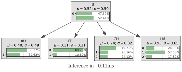
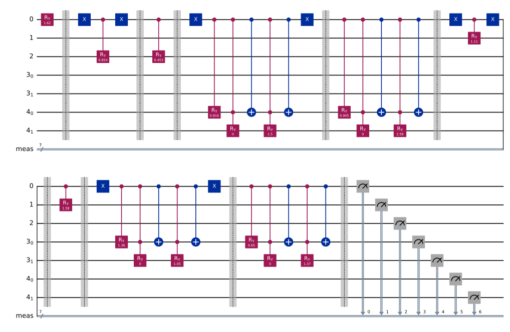
Variables with more than 2 states require \(\lceil \log_2(|\text{dom}|) \rceil > 1\) qubits. Here node B has 2 states and several children have 3 states (2 qubits each).
In [14]:
bn_bk = gum.fastBN("B->AU; B->IT; B->CH[3]; B->LM[3]")
bn_bk.generateCPTs()
gnb.showInference(bn_bk)
In [15]:
qbn_bk = qBNS.qBNMC(bn_bk)
print(f"Total qubits: {qbn_bk.getTotNumQBits()}")
print(f"Qubit widths: { {bn_bk.variable(n).name(): qbn_bk.getWidth(n) for n in bn_bk.nodes()} }")
qbn_bk.buildCircuit().draw("mpl", scale=0.6)
Total qubits: 7
Qubit widths: {'B': 1, 'AU': 1, 'IT': 1, 'CH': 2, 'LM': 2}
Out[15]:
In [16]:
marginals_bk = qbn_bk.runBN(shots=10000)

ie_bk = gum.LazyPropagation(bn_bk)
ie_bk.makeInference()

gnb.sideBySide(
  marginals_bk["CH"],
  ie_bk.posterior("CH"),
  captions=["qBNMC — 10 000 shots", "LazyPropagation — exact"],
)
Part 2 — qBNRejection: inference with evidence
qBNRejection implements quantum rejection sampling (Low et al., 2014). Given evidence \(e\), it uses the Grover iterate \(G = S_e \, A^{-1} \, S_0 \, A\) to amplify the amplitude of states consistent with \(e\), where:
\(A\) is the quantum circuit encoding of the BN (built by
qBNMC);\(S_e\) is a phase flip on the evidence qubits;
\(S_0\) is a phase flip on the all-zero state.
Each call to getSample applies \(G^{\lceil 2^k \rceil}\) for increasing \(k\) until a measurement consistent with the evidence is obtained (Algorithm 1). makeInference accumulates max_iter such samples to estimate the posterior.
Basic usage: 3-node BN with evidence
In [17]:
bn = gum.fastBN("A->B<-C", 2)
evidence = {"B": 0}

# Exact reference
ie = gum.LazyPropagation(bn)
ie.setEvidence(evidence)
ie.makeInference()
print("Exact P(A | B=0):", ie.posterior("A"))
Exact P(A | B=0):
  A                │
0        │1        │
─────────│─────────│
 0.2039  │ 0.7961  │
In [18]:
qbn = qBNS.qBNMC(bn)
qinf = qBNS.qBNRejection(qbn)
qinf.setEvidence(evidence)
qinf.setMaxIter(500)
qinf.makeInference()
Out[18]:
{'A': [0.20800000000000016, 0.7920000000000006],
 'B': [1.0000000000000007, 0.0],
 'C': [0.9020000000000007, 0.09800000000000007]}
In [19]:
gnb.sideBySide(
  qinf.posterior("A"),
  ie.posterior("A"),
  captions=["qBNRejection — 500 samples", "LazyPropagation — exact"],
)
Restricting to the relevant subgraph: useFragmentBN
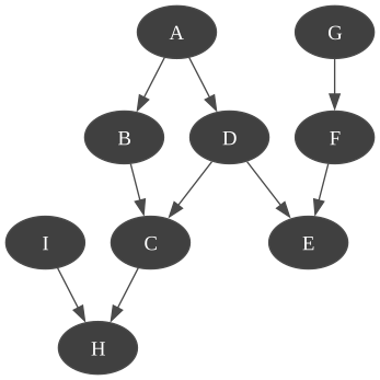
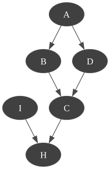
For a query involving only a subset of nodes, useFragmentBN builds a minimal BayesNetFragment containing only the ancestors of the target and evidence nodes. This reduces the number of qubits and speeds up the circuit.
In [20]:
# Larger BN: A->B->C->H; I->H; A->D->C; D->E; G->F->E
bn_large = gum.fastBN("A->B->C->H;I->H;A->D->C;D->E;G->F->E", 2)
gnb.showBN(bn_large, size=8)
In [21]:
evidence_large = {"H": 0, "A": 1}
target = "D"

qbn_large = qBNS.qBNMC(bn_large)
qinf_large = qBNS.qBNRejection(qbn_large)
qinf_large.setEvidence(evidence_large)

# Restrict the circuit to the ancestors of {target} ∪ evidence
qinf_large.useFragmentBN(target={target})

print(f"Full BN: {bn_large.size()} nodes, {qbn_large.getTotNumQBits()} qubits")
print(f"Fragment: {qinf_large.qbn.bn.size()} nodes, {qinf_large.qbn.getTotNumQBits()} qubits")
gnb.showBN(qinf_large.qbn.bn)
Full BN: 9 nodes, 9 qubits
Fragment: 6 nodes, 6 qubits
In [22]:
qinf_large.setMaxIter(500)
qinf_large.makeInference()

ie_large = gum.LazyPropagation(bn_large)
ie_large.setEvidence(evidence_large)
ie_large.makeInference()

gnb.sideBySide(
  qinf_large.posterior(target),
  ie_large.posterior(target),
  captions=[f"qBNRejection — P({target} | H=0, A=1)", "LazyPropagation — exact"],
)
Named example: 4-node Oil BN with evidence
In [23]:
bn_oil = gum.fastBN("IR->SM->SP<-OI", 2)
bn_oil.cpt("IR")[:] = [0.75, 0.25]
bn_oil.cpt("SM")[:] = [[0.3, 0.7], [0.8, 0.2]]
bn_oil.cpt("OI")[:] = [0.6, 0.4]
bn_oil.cpt("SP")[:] = [[[0.1, 0.9], [0.3, 0.7]], [[0.4, 0.6], [0.7, 0.3]]]

evidence_oil = {"SP": 1}
target_oil = "OI"

ie_oil = gum.LazyPropagation(bn_oil)
ie_oil.setEvidence(evidence_oil)
ie_oil.makeInference()
print(f"Exact P({target_oil} | SP=1) = {ie_oil.posterior(target_oil)}")
Exact P(OI | SP=1) =
  OI               │
0        │1        │
─────────│─────────│
 0.7336  │ 0.2664  │
In [24]:
qbn_oil = qBNS.qBNMC(bn_oil)
qinf_oil = qBNS.qBNRejection(qbn_oil)
qinf_oil.setEvidence(evidence_oil)
qinf_oil.useFragmentBN(target={target_oil})
qinf_oil.setMaxIter(500)
qinf_oil.makeInference()

gnb.sideBySide(
  qinf_oil.posterior(target_oil),
  ie_oil.posterior(target_oil),
  captions=[f"qBNRejection — P({target_oil} | SP=1)", "LazyPropagation — exact"],
)
QBN Summary
Class |
Purpose |
Key method |
|---|---|---|
|
Encode BN as quantum circuit |
|
|
Posterior inference with evidence |
|
Useful workflow:
Build
qBNMC(bn)— circuit encoding.Check marginals via
runBN()(no evidence).Build
qBNRejection(qbn)and calluseFragmentBN(target, evidence)to reduce circuit size.setEvidence(),setMaxIter(),makeInference(),posterior(node).
In [ ]: