Credal Networks

In [1]:

import matplotlib.pyplot as plt

import pyagrum.credal_net as gum
import pyagrum.lib.notebook as gnb

gnb.configuration()

Library	Version
OS	posix [darwin]
Python	3.14.7 (main, Aug 5 2026, 10:29:49) [Clang 21.0.0 (clang-2100.1.1.101)]
IPython	9.17.1
Matplotlib	3.11.2
Numpy	2.5.3
pyDot	4.0.1
pyAgrum	3.2.0

Mon Sep 28 17:47:26 2026 CEST

Credal Net from BN

In [2]:

bn = gum.fastBN("A->B[3]->C<-D<-A->E->F")
bn_min = gum.BayesNet(bn)
bn_max = gum.BayesNet(bn)
for n in bn.nodes():
  x = 0.4 * min(bn.cpt(n).min(), 1 - bn.cpt(n).max())
  bn_min.cpt(n).translate(-x)
  bn_max.cpt(n).translate(x)

cn = gum.CredalNet(bn_min, bn_max)
cn.intervalToCredal()
cn

Out[2]:

inference on Credal Net

In [3]:

gnb.flow.row(
  bn, bn.cpt("B"), cn, bn_min.cpt("B"), bn_max.cpt("B"), captions=["Bayes Net", "CPT", "Credal Net", "CPTmin", "CPTmax"]
)

Out[3]:

Bayes Net

	B
A	0	1	2
0	0.5969	0.3795	0.0236
1	0.3938	0.5270	0.0792

CPT

Credal Net

	B
A	0	1	2
0	0.5874	0.3701	0.0142
1	0.3844	0.5175	0.0698

CPTmin

	B
A	0	1	2
0	0.6063	0.3890	0.0331
1	0.4033	0.5364	0.0887

CPTmax

Binarization

We can use LBP on CN (L2U) only for binary credal networks (here B is not binary). We then propose the classical binarization (but warn the user that this leads to approximation in the inference)

In [4]:

cn2 = gum.CredalNet(bn_min, bn_max)
cn2.intervalToCredal()
cn2.approximatedBinarization()
cn2.computeBinaryCPTMinMax()

gnb.flow.row(cn, cn2, captions=["Credal net", "Binarized credal net"])

Out[4]:

Credal net

Binarized credal net

Here, \(B\) becomes

\(B\)-b\(i\) : the \(i\)-th bit of B
instrumental \(B\)-v\(k\) : the indicator variable for each modality \(k\) of \(B\)

In [5]:

ie_mc = gum.CNMonteCarloSampling(cn)
ie2_lbp = gum.CNLoopyPropagation(cn2)
ie2_mc = gum.CNMonteCarloSampling(cn2)

In [6]:

gnb.sideBySide(
  gnb.getInference(cn, engine=ie_mc), gnb.getInference(cn2, engine=ie2_mc), gnb.getInference(cn2, engine=ie2_lbp)
)

In [7]:

gnb.sideBySide(
  ie_mc.CN(),
  ie_mc.marginalMin("F"),
  ie_mc.marginalMax("F"),
  ie_mc.CN(),
  ie2_lbp.marginalMin("F"),
  ie2_lbp.marginalMax("F"),
  ncols=3,
)
print(cn)

F
0	1
0.5842	0.2667

F
0	1
0.7333	0.4158

F
0	1
0.5643	0.2667

F
0	1
0.7333	0.4357


A:Range([0,1])
<> : [[0.596302 , 0.403698] , [0.826986 , 0.173014]]

B:Range([0,2])
<A:0> : [[0.587421 , 0.379505 , 0.0330739] , [0.587421 , 0.388956 , 0.023623] , [0.596871 , 0.388956 , 0.0141732] , [0.606319 , 0.379507 , 0.0141732] , [0.59687 , 0.370056 , 0.0330739] , [0.606319 , 0.370056 , 0.0236241]]
<A:1> : [[0.384359 , 0.526956 , 0.088685] , [0.384359 , 0.536406 , 0.0792351] , [0.393808 , 0.536406 , 0.0697865] , [0.403259 , 0.526955 , 0.0697865] , [0.393809 , 0.517506 , 0.088685] , [0.403259 , 0.517506 , 0.0792349]]

C:Range([0,1])
<B:0|D:0> : [[0.472727 , 0.527273] , [0.620529 , 0.379471]]
<B:1|D:0> : [[0.713883 , 0.286117] , [0.861685 , 0.138315]]
<B:2|D:0> : [[0.274834 , 0.725166] , [0.422636 , 0.577364]]
<B:0|D:1> : [[0.741346 , 0.258654] , [0.889148 , 0.110852]]
<B:1|D:1> : [[0.428827 , 0.571173] , [0.576628 , 0.423372]]
<B:2|D:1> : [[0.435561 , 0.564439] , [0.583364 , 0.416636]]

D:Range([0,1])
<A:0> : [[0.691702 , 0.308298] , [0.817262 , 0.182738]]
<A:1> : [[0.0941685 , 0.905832] , [0.219728 , 0.780272]]

E:Range([0,1])
<A:0> : [[0.358324 , 0.641676] , [0.471637 , 0.528363]]
<A:1> : [[0.0849858 , 0.915014] , [0.198298 , 0.801702]]

F:Range([0,1])
<E:0> : [[0.801695 , 0.198305] , [0.915011 , 0.084989]]
<E:1> : [[0.486038 , 0.513962] , [0.599356 , 0.400644]]

Credal Net from bif files

In [8]:

cn = gum.CredalNet("res/cn/2Umin.bif", "res/cn/2Umax.bif")
cn.intervalToCredal()

In [9]:

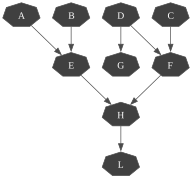
gnb.showCN(cn, "2")

../_images/notebooks_24-Models_credalNetworks_15_0.svg

In [10]:

ie = gum.CNMonteCarloSampling(cn)
ie.insertEvidenceFile("res/cn/L2U.evi")

In [11]:

ie.setRepetitiveInd(False)
ie.setMaxTime(1)
ie.setMaxIter(1000)

ie.makeInference()

In [12]:

cn

Out[12]:

In [13]:

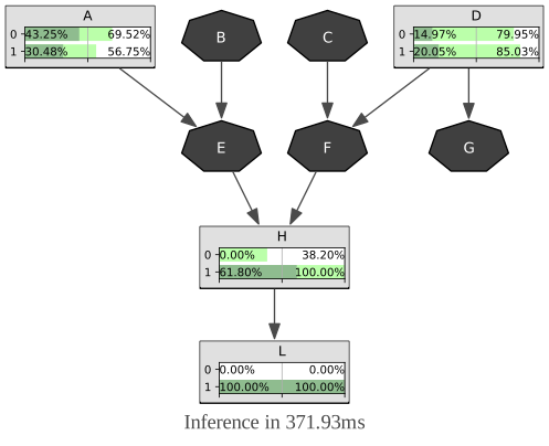
gnb.showInference(cn, targets={"A", "H", "L", "D"}, engine=ie, evs={"L": [0, 1], "G": [1, 0]})

../_images/notebooks_24-Models_credalNetworks_19_0.svg

Comparing inference in credal networks

In [14]:

import pyagrum.credal_net as gum


def showDiffInference(model, mc, lbp):
  for i in model.current_bn().nodes():
    a, b = mc.marginalMin(i)[:]
    c, d = mc.marginalMax(i)[:]

    e, f = lbp.marginalMin(i)[:]
    g, h = lbp.marginalMax(i)[:]

    plt.scatter([a, b, c, d], [e, f, g, h])


cn = gum.CredalNet("res/cn/2Umin.bif", "res/cn/2Umax.bif")
cn.intervalToCredal()

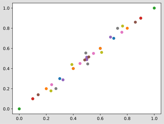
Inference with no evidence

The two inference give quite the same result

In [15]:

ie_mc = gum.CNMonteCarloSampling(cn)
ie_mc.makeInference()

cn.computeBinaryCPTMinMax()
ie_lbp = gum.CNLoopyPropagation(cn)
ie_lbp.makeInference()

showDiffInference(cn, ie_mc, ie_lbp)

../_images/notebooks_24-Models_credalNetworks_23_0.svg

The problem of evidence

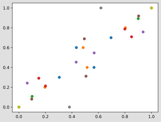
When evidence are inserted, there are some divergence.

In [16]:

ie_mc = gum.CNMonteCarloSampling(cn)
ie_mc.insertEvidenceFile("res/cn/L2U.evi")
ie_mc.makeInference()

ie_lbp = gum.CNLoopyPropagation(cn)
ie_lbp.insertEvidenceFile("res/cn/L2U.evi")
ie_lbp.makeInference()

showDiffInference(cn, ie_mc, ie_lbp)

../_images/notebooks_24-Models_credalNetworks_25_0.svg

Dynamical Credal Net

In [17]:

cn = gum.CredalNet("res/cn/bn_c_8.bif", "res/cn/den_c_8.bif")
cn.bnToCredal(0.8, False)

In [18]:

ie = gum.CNMonteCarloSampling(cn)
ie.insertModalsFile("res/cn/modalities.modal")

ie.setRepetitiveInd(True)
ie.setMaxTime(5)
ie.setMaxIter(1000)

ie.makeInference()

In [19]:

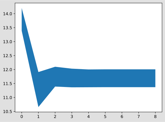
print(ie.dynamicExpMax("temp"))

(14.203404648128334, 11.911090684366485, 12.10019505553209, 12.031555584857191, 12.003107180947513, 12.007979271958872, 12.007860641421736, 12.007652604938034, 12.007725006693335)

In [20]:

fig = plt.figure()
ax = fig.add_subplot(111)
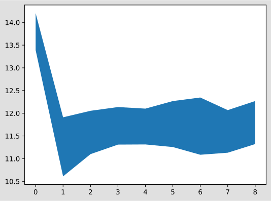
ax.fill_between(range(9), ie.dynamicExpMax("temp"), ie.dynamicExpMin("temp"))
plt.show()

../_images/notebooks_24-Models_credalNetworks_30_0.svg

In [21]:

ie = gum.CNMonteCarloSampling(cn)
ie.insertModalsFile("res/cn/modalities.modal")

ie.setRepetitiveInd(False)
ie.setMaxTime(5)
ie.setMaxIter(1000)

ie.makeInference()
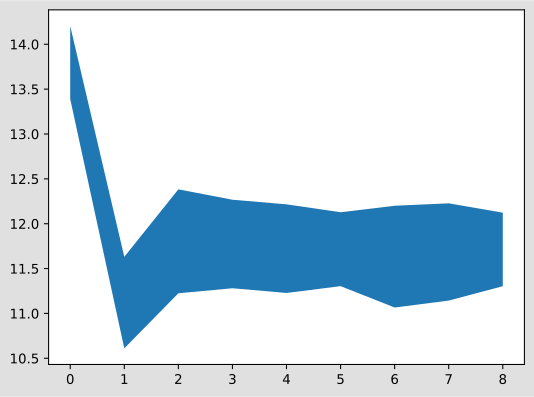
print(ie.messageApproximationScheme())

stopped with epsilon=0

In [22]:

fig = plt.figure()
ax = fig.add_subplot(111)
ax.fill_between(range(9), ie.dynamicExpMax("temp"), ie.dynamicExpMin("temp"))
plt.show()

../_images/notebooks_24-Models_credalNetworks_32_0.svg

In [23]:

ie = gum.CNMonteCarloSampling(cn)
ie.insertModalsFile("res/cn/modalities.modal")

ie.setRepetitiveInd(False)
ie.setMaxTime(5)
ie.setMaxIter(5000)

gnb.animApproximationScheme(ie)
ie.makeInference()

../_images/notebooks_24-Models_credalNetworks_33_0.svg

../_images/notebooks_24-Models_credalNetworks_33_1.svg

In [24]:

fig = plt.figure()
ax = fig.add_subplot(111)
ax.fill_between(range(9), ie.dynamicExpMax("temp"), ie.dynamicExpMin("temp"))
plt.show()

../_images/notebooks_24-Models_credalNetworks_34_0.svg

In [ ]: