Markov random fields (a.k.a. Markov Networks)
|
|
|



In [1]:
import pyagrum.markov_random_field as gum
import pyagrum.lib.notebook as gnb
import pyagrum.lib.mrf2graph as m2g
building a Markov random field
In [2]:
gum.config.reset()  # back to default
gum.config["notebook", "default_markovrandomfield_view"] = "graph"
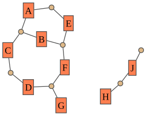
mn = gum.fastMRF("A--B--C;C--D;B--E--F;F--D--G;H--J;E--A;J")
mn
Out[2]:
Using pyagrum.config, it is possible to adapt the graphical representations for Markov random field (see the notebook 99-Tools_configForPyAgrum.ipynb).
In [3]:
gum.config.reset()  # back to default
gum.config["factorgraph", "edge_length"] = "0.4"
gnb.showMRF(mn)
In [4]:
gum.config.reset()  # back to default
print("Default view for Markov random field: " + gum.config["notebook", "default_markovrandomfield_view"])
gum.config["notebook", "default_markovrandomfield_view"] = "graph"
print("modified to: " + gum.config["notebook", "default_markovrandomfield_view"])
mn
Default view for Markov random field: factorgraph
modified to: graph
Out[4]:
In [5]:
gnb.sideBySide(gnb.getMRF(mn, view="graph", size="5"), gnb.getMRF(mn, view="factorgraph", size="5"))
In [6]:
gnb.showMRF(mn)
print(mn)
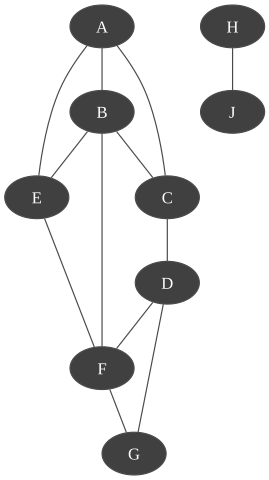
MRF{nodes: 9, edges: 12, domainSize: 512, dim: 38}
Accessors for Markov random fields
In [7]:
print(f"nodes       : {mn.nodes()}")
print(f"node names  : {mn.names()}")
print(f"edges       : {mn.edges()}")
print(f"components  : {mn.connectedComponents()}")
print(f"factors     : {mn.factors()}")
print(f"factor(C,D) : {mn.factor({2, 3})}")
print(f"factor(C,D) : {mn.factor({'C', 'D'})}")
nodes       : {0, 1, 2, 3, 4, 5, 6, 7, 8}
node names  : {'F', 'J', 'H', 'B', 'G', 'E', 'D', 'C', 'A'}
edges       : {(0, 1), (1, 2), (0, 4), (1, 5), (1, 4), (2, 3), (4, 5), (0, 2), (5, 6), (7, 8), (3, 6), (3, 5)}
components  : {3: 0, 8: 1, 1: 0, 6: 0, 4: 0, 7: 1, 0: 0, 2: 0, 5: 0}
factors     : [{0, 1, 2}, {2, 3}, {8, 7}, {1, 4, 5}, {3, 5, 6}, {0, 4}, {8}]
factor(C,D) :
      ║  C                │
D     ║0        │1        │
──────║─────────│─────────│
0     ║ 0.8909  │ 0.6650  │
1     ║ 0.1209  │ 0.8861  │

factor(C,D) :
      ║  C                │
D     ║0        │1        │
──────║─────────│─────────│
0     ║ 0.8909  │ 0.6650  │
1     ║ 0.1209  │ 0.8861  │
In [8]:
try:
  mn.factor({0, 1})
except gum.GumException as e:
  print(e)
try:
  mn.factor({"A", "B"})
except gum.GumException as e:
  print(e)
[pyAgrum] Object not found: No element with the key <{1,0}>
[pyAgrum] Object not found: No element with the key <{1,0}>
Manipulating factors
In [9]:
mn.factor({"A", "B", "C"})
Out[9]:
|
|
| ||
|---|---|---|---|
|
| 0.7067 | 0.8253 | |
| 0.8746 | 0.5398 | ||
|
| 0.0879 | 0.7562 | |
| 0.5665 | 0.7454 | ||
In [10]:
mn.factor({"A", "B", "C"})[{"B": 0}]
Out[10]:
array([[0.70671783, 0.82529402],
       [0.087854  , 0.75624566]])
In [11]:
mn.factor({"A", "B", "C"})[{"B": 0}] = [[1, 2], [3, 4]]
mn.factor({"A", "B", "C"})
Out[11]:
|
|
| ||
|---|---|---|---|
|
| 1.0000 | 2.0000 | |
| 0.8746 | 0.5398 | ||
|
| 3.0000 | 4.0000 | |
| 0.5665 | 0.7454 | ||
Customizing graphical representation
In [12]:
gum.config.reset()  # back to default
gum.config["factorgraph", "edge_length"] = "0.5"

maxnei = max([len(mn.neighbours(n)) for n in mn.nodes()])
nodemap = {n: len(mn.neighbours(mn.idFromName(n))) / maxnei for n in mn.names()}

facmax = max([len(f) for f in mn.factors()])
fgma = lambda factor: (1 + len(factor) ** 2) / (1 + facmax * facmax)

gnb.flow.row(
  gnb.getGraph(m2g.MRF2UGdot(mn)),
  gnb.getGraph(m2g.MRF2UGdot(mn, nodeColor=nodemap)),
  gnb.getGraph(m2g.MRF2FactorGraphdot(mn)),
  gnb.getGraph(m2g.MRF2FactorGraphdot(mn, factorColor=fgma, nodeColor=nodemap)),
  captions=[
    "Markov random field",
    "MarkovRandomField with colored node w.r.t number of neighbours",
    "MarkovRandomField as factor graph",
    "MRF with colored factor w.r.t to the size of scope",
  ],
)
Out[12]:
from BayesNet to MarkovRandomField
In [13]:
bn = gum.fastBN("A->B<-C->D->E->F<-B<-G;A->H->I;C->J<-K<-L")
mn = gum.MarkovRandomField.fromBN(bn)
gnb.flow.row(
  bn, gnb.getGraph(m2g.MRF2UGdot(mn)), captions=["a Bayesian network", "the corresponding Markov random field"]
)
Out[13]:
In [14]:
# The corresponding factor graph
m2g.MRF2FactorGraphdot(mn)
Out[14]:
Inference in Markov random field
In [15]:
bn = gum.fastBN("A->B<-C->D->E->F<-B<-G;A->H->I;C->J<-K<-L")
iebn = gum.LazyPropagation(bn)

mn = gum.MarkovRandomField.fromBN(bn)
iemn = gum.ShaferShenoyMRFInference(mn)
iemn.setEvidence({"A": 1, "F": [0.4, 0.8]})
iemn.makeInference()
iemn.posterior("B")
Out[15]:
|
|
|
|---|---|
| 0.1362 | 0.8638 |
In [16]:
def affAGC(evs):
  gnb.sideBySide(
    gnb.getSideBySide(
      gum.getPosterior(bn, target="A", evs=evs),
      gum.getPosterior(bn, target="G", evs=evs),
      gum.getPosterior(bn, target="C", evs=evs),
    ),
    gnb.getSideBySide(
      gum.getPosterior(mn, target="A", evs=evs),
      gum.getPosterior(mn, target="G", evs=evs),
      gum.getPosterior(mn, target="C", evs=evs),
    ),
    captions=[
      "Inference in the Bayesian network bn with evidence " + str(evs),
      "Inference in the Markov random field mn with evidence " + str(evs),
    ],
  )


print(
  "Inference for both the corresponding models in BayesNet and Markov Random Field worlds when the MRF comes from a BN"
)
affAGC({})
print("C has no impact on A and G")
affAGC({"C": 1})

print("But if B is observed")
affAGC({"B": 1})
print("C has an impact on A and G")
affAGC({"B": 1, "C": 0})
Inference for both the corresponding models in BayesNet and Markov Random Field worlds when the MRF comes from a BN
C has no impact on A and G
But if B is observed
C has an impact on A and G
In [17]:
mn.generateFactors()
print("But with more general factors")
affAGC({})
print("C has impact on A and G even without knowing B")
affAGC({"C": 1})
But with more general factors
C has impact on A and G even without knowing B
Graphical inference in Markov random field
In [18]:
bn = gum.fastBN("A->B<-C->D->E->F<-B<-G;A->H->I;C->J<-K<-L")
mn = gum.MarkovRandomField.fromBN(bn)

gnb.sideBySide(
  gnb.getJunctionTree(bn),
  gnb.getJunctionTree(mn),
  captions=["Junction tree for the BN", "Junction tree for the induced MN"],
)
gnb.sideBySide(
  gnb.getJunctionTreeMap(bn, size="3!"),
  gnb.getJunctionTreeMap(mn, size="3!"),
  captions=["Map of the junction tree for the BN", "Map of the junction tree for the induced MN"],
)
In [19]:
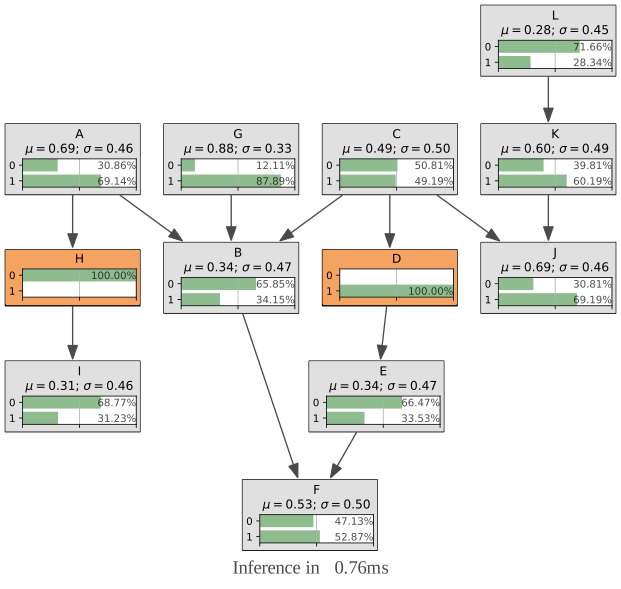
gnb.showInference(bn, evs={"D": 1, "H": 0})
In [20]:
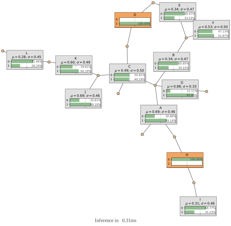
gum.config.reset()
gnb.showInference(mn, size="8", evs={"D": 1, "H": 0})
In [21]:
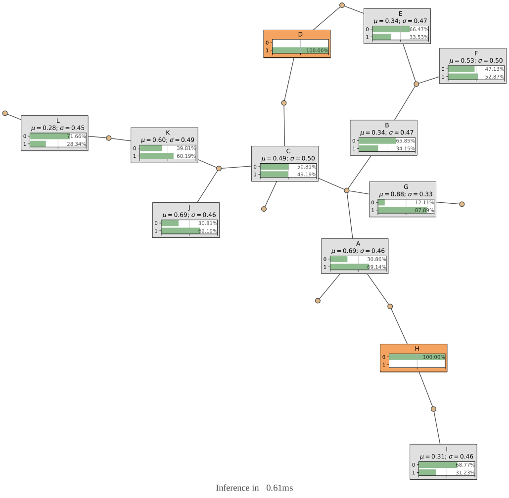
gum.config["factorgraph", "edge_length_inference"] = "1.1"
gnb.showInference(mn, size="11", evs={"D": 1, "H": 0})
In [22]:
gum.config["notebook", "default_markovrandomfield_view"] = "graph"
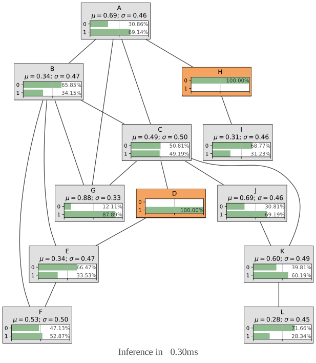
gnb.showInference(mn, size="8", evs={"D": 1, "H": 0})