Using k-order Dynamic Bayesian Networks (k-TBN)

A k-TBN (k-order dynamic Bayesian network) generalizes the classical 2-TBN: instead of letting a variable at time \(t\) depend on a single step backward, it lets it depend on up to the \(k\) most recent time slices. A k-TBN is a template of \(k\) consecutive slices; unrolling it for any horizon \(T \geq k\) produces a plain pyagrum.BayesNet.

A k-TBN distinguishes two kinds of variables:

• temporal variables (processes), which evolve through time and have one instance per slice,

• atemporal variables, constant through time (e.g. a static context), which have a single instance.

(For more details see https://pyagrum.readthedocs.io/en/latest/ktbn.html)

import pyagrum as gum
import pyagrum.lib.notebook as gnb
import pyagrum.ktbn as ktbn

Building a k-TBN by hand

A small weather example: whether it Rains and whether an Umbrella is carried depend on the previous time slice, and both depend on the (atemporal) Season. Rain and Umbrella are added as temporal processes (one instance per slice); Season is added as atemporal (a single instance, addressed with ktbn.KTBN.ATEMPORAL).

m = ktbn.KTBN(2)  # k=2: each variable depends on at most the previous slice

m.addTemporal(gum.LabelizedVariable("Rain", "raining?", ["no", "yes"]))
m.addTemporal(gum.LabelizedVariable("Umbrella", "umbrella carried?", ["no", "yes"]))
m.addAtemporal(gum.LabelizedVariable("Season", "season", ["dry", "wet"]))

m.addArc("Season", ktbn.KTBN.ATEMPORAL, "Rain", 0)
m.addArc("Season", ktbn.KTBN.ATEMPORAL, "Rain", 1)
m.addArc("Rain", 0, "Rain", 1)
m.addArc("Rain", 0, "Umbrella", 0)
m.addArc("Rain", 1, "Umbrella", 1)
m

Nodes can be addressed either by an explicit (base, slice) pair, or by their engine name using bracket notation ("Rain[1]" for Rain at slice 1, a bare name like "Season" for an atemporal variable). Both spellings are accepted almost everywhere, including toDot()’s slice-clustered rendering below.

fillCPT fills one conditional distribution at a time, addressing the node and its parents by name instead of by CPT positional order – convenient once a k-TBN has more than a couple of parents per node. When the target node is given as "base[slice]", parent keys can freely mix engine names and (base, slice) tuples; when the target is given as a (base, slice) pair instead, every parent key must also be a tuple.

m.fillCPT("Season", ktbn.KTBN.ATEMPORAL, {}, [0.5, 0.5])

m.fillCPT("Rain[0]", {"Season": "dry"}, [0.9, 0.1])
m.fillCPT("Rain[0]", {"Season": "wet"}, [0.4, 0.6])
m.fillCPT("Rain[1]", {"Rain[0]": "no", "Season": "dry"}, [0.8, 0.2])
m.fillCPT("Rain[1]", {"Rain[0]": "yes", "Season": "dry"}, [0.5, 0.5])
m.fillCPT("Rain[1]", {"Rain[0]": "no", "Season": "wet"}, [0.3, 0.7])
m.fillCPT("Rain[1]", {"Rain[0]": "yes", "Season": "wet"}, [0.1, 0.9])

m.fillCPT("Umbrella[0]", {"Rain[0]": "no"}, [0.9, 0.1])
m.fillCPT("Umbrella[0]", {"Rain[0]": "yes"}, [0.2, 0.8])
m.fillCPT("Umbrella[1]", {"Rain[1]": "no"}, [0.9, 0.1])
m.fillCPT("Umbrella[1]", {"Rain[1]": "yes"}, [0.2, 0.8])

m.cpt("Rain[1]")

		Rain[1]
Rain[0]	Season	no	yes
no	dry	0.8000	0.2000
	wet	0.3000	0.7000
yes	dry	0.5000	0.5000
	wet	0.1000	0.9000

The same fast-construction syntax as pyagrum.fastBN is available through gum.fastVariable, using bracket notation to declare a process’s domain directly in its name ("X[2]"): add() clones it into k instances unless temporal=False is passed.

m2 = ktbn.KTBN(2)
m2.add(gum.fastVariable("X[2]"))  # temporal by default: X[0], X[1]
m2.add(gum.fastVariable("C"), False)  # atemporal
m2.addArc("X", 0, "X", 1)
m2.addArc("C", ktbn.KTBN.ATEMPORAL, "X", 0)
m2.generateCPTs()  # random CPTs, useful for quick experiments
m2

Unrolling into a plain Bayesian network

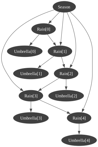
unroll(T) expands the template into a standard pyagrum.BayesNet with exactly T time slices: slices 0..k-1 are copied verbatim, every later slice replicates the transition kernel (slice k-1). The result can be used with any of pyAgrum’s usual BN inference engines.

bn = m.unroll(5)
gnb.showBN(bn, size="6")

ie = gum.LazyPropagation(bn)
ie.makeInference()
ie.posterior("Rain[3]")

Rain[3]
no	yes
0.4233	0.5768

Inference directly on the k-TBN

KTBNInference runs inference over the k-TBN template directly, without materializing the unrolled network. It supports hard/soft observations, do-interventions, and both are addressed the same way as everywhere else: (base, slice) or an engine name.

kie = ktbn.KTBNInference(m)
kie.addObservation("Season", "wet")
kie.addObservation("Rain", 0, "yes")
kie.makeInference(5)  # horizon: number of time slices to compute

kie.posterior("Rain", 3)

Rain[3]
no	yes
0.1240	0.8760

# the whole time series for one base variable, one Tensor per slice
series = kie.posteriors("Rain")
for t, p in enumerate(series):
  print(f"P(Rain[{t}] | Season=wet, Rain[0]=yes) =", p.tolist())

P(Rain[0] | Season=wet, Rain[0]=yes) = [0.0, 1.0]
P(Rain[1] | Season=wet, Rain[0]=yes) = [0.09999999999999998, 0.8999999999999999]
P(Rain[2] | Season=wet, Rain[0]=yes) = [0.11999999999999998, 0.8799999999999999]
P(Rain[3] | Season=wet, Rain[0]=yes) = [0.124, 0.8759999999999999]
P(Rain[4] | Season=wet, Rain[0]=yes) = [0.12480000000000002, 0.8752]

addIntervention sets a variable by do(...) instead of conditioning on it – the causal semantics differ from an observation whenever the intervened variable has parents in the template.

kie2 = ktbn.KTBNInference(m)
kie2.addIntervention("Rain", 0, "yes")  # do(Rain[0] = yes), regardless of Season
kie2.makeInference(4)
kie2.posterior("Umbrella", 3)

Umbrella[3]
no	yes
0.4867	0.5134

print("In dry season")
gnb.plotFollowKTBN(
  m,
  ["Rain", "Umbrella"],
  T=51,
  observations={"Rain[0]": "yes", "Rain[16]": "no", "Rain[40]": "yes", "Season": "dry"},
)
print("In wet season")
gnb.plotFollowKTBN(
  m,
  ["Rain", "Umbrella"],
  T=51,
  observations={"Rain[0]": "yes", "Rain[16]": "no", "Rain[40]": "yes", "Season": "wet"},
)

In dry season

In wet season

Persistence

A k-TBN is saved/loaded through save/load (or the free functions saveKTBN/loadKTBN), in a text (.jgum) or binary (.bgum) GUM format selected by the file extension. Bracket-encoded engine names are preserved literally through the round-trip, including nested brackets such as "X[0][2]" for a fast-syntax process named X[2] at slice 0.

import tempfile, os

path = os.path.join(tempfile.mkdtemp(), "weather.bgum")
m.save(path)
reloaded = ktbn.loadKTBN(path)
print(reloaded.k(), reloaded.sizeArcs())

2 5

Randomly generating a k-TBN

KTBNGenerator draws a random template – variables, a legal arc set, and (optionally) random CPTs – mainly to build ground-truth models for learning experiments: sample trajectories, learn the structure back, and compare.

gum.initRandom(42)
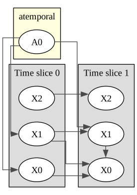
gen = ktbn.KTBNGenerator(2, 3, 1)  # k=2, 3 temporal processes, 1 atemporal variable
gen.setDensity(0.4)
gm = gen.generate()
gm.generateCPTs()
gnb.showDot(gm.toDot())

Sampling trajectories and learning a k-TBN back

Unlike a plain Bayesian network, a k-TBN describes a process: its database is a set of trajectories, one CSV file per trajectory, rather than a flat table of i.i.d. rows. KTBNDatabaseGenerator samples them by sliding the k-slice template forward in time.

dbgen = ktbn.KTBNDatabaseGenerator(gm)
outdir = tempfile.mkdtemp()
dbgen.drawSamples(10, 120, outdir, "traj")  # 10 trajectories of length 120

(-282.24371441397096,
 -308.0567440707682,
 -293.54535129567455,
 -291.2278161482233,
 -276.9192265508581,
 -288.42208135415683,
 -307.31491937086685,
 -287.4236881178443,
 -293.16824903148415,
 -285.411951340677)

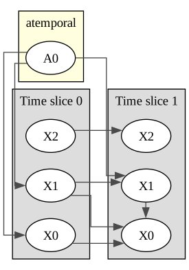
KTBNLearner learns the order-k structure and parameters back from the trajectories. Domains are inferred from the first trajectory by default, which is unsafe for atemporal columns (constant within a trajectory, so only one label ever shows up in file 1): supplying a schema BayesNet with the full domains sidesteps that.

dbgen.drawSamples(200, 100, outdir, "traj")  # 200 trajectories of length 100

schema = gum.BayesNet()
for name in list(gm.temporalVarNames()) + list(gm.atemporalVarNames()):
  schema.add(gum.LabelizedVariable(name, "", ["0", "1"]))

learner = ktbn.KTBNLearner(outdir, "traj", 200, 2, schema, gm.atemporalVarNames())
learner.useScoreBIC().useGreedyHillClimbing()
learned = learner.learnKTBN()
gnb.showDot(learned.toDot())

When the order \(k\) itself is unknown, KTBNAdaptiveLearner explores every candidate in [2, kMax], learns one k-TBN per candidate, and keeps the one with the best cross-\(k\) model-selection score (BIC by default).

adaptive = ktbn.KTBNAdaptiveLearner(outdir, "traj", 200, 5, schema, gm.atemporalVarNames())
adaptive.useScoreBIC().useGreedyHillClimbing()
best = adaptive.learnKTBN()
print("selected k :", adaptive.bestK())
print("score per candidate k :", adaptive.scorePerCandidateK())

selected k : 2
score per candidate k : ((2, -48749.842130120516), (3, -48806.847471629546), (4, -48874.07945582724), (5, -48945.778281573796))

Multi-lag order and the summary graph

A k-TBN can depend on more than one lag at once: nothing forces the transition kernel to draw all its parents from the immediately preceding slice. This example builds a k=4 model with three temporal processes A, B, C, where A depends on two different lags – A[0] (lag 3) and A[2] (lag 1) – combined so that A behaves as a 4-bit Fibonacci LFSR (linear-feedback shift register): A[3] is (almost) the XOR of A[0] and A[2], a classic recipe for a long pseudo-random binary sequence. B and C relay that signal one lag at a time, so its effect propagates visibly through the whole network.

Fixed CPTs are used on purpose to get a reproducible, interesting dynamic rather than noise.

m = ktbn.KTBN(4)  # k=4

for name in ["A", "B", "C"]:
  m.addTemporal(gum.LabelizedVariable(name, "", ["0", "1"]))

# A[3] depends on two different lags: A[0] (lag 3) and A[2] (lag 1)
m.addArc("A", 0, "A", 3)
m.addArc("A", 2, "A", 3)

# B and C relay the signal one lag at a time
m.addArc("A", 2, "B", 3)
m.addArc("B", 2, "B", 3)
m.addArc("B", 2, "C", 3)
m.addArc("C", 2, "C", 3)

# Between t=1 and t=1 : a prior for C[0]-A[1]
m.addArc("C", 0, "A", 1)

gnb.show(m)

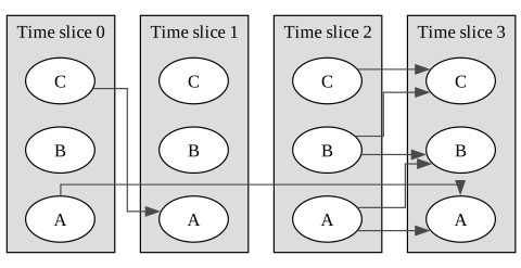
A[3] is fixed as a noisy XOR of its two lagged parents – the LFSR feedback – while B and C each mix their own lag-1 persistence with the upstream signal:

# A: initial slices are an unconstrained (uniform) seed for the LFSR
# for t in range(3):
#  m.fillCPT("A", t, {}, [0.5, 0.5])
m.generateCPTs()

# A[3] = noisy XOR(A[0], A[2]): the LFSR feedback
m.fillCPT("A", 3, {("A", 0): "0", ("A", 2): "0"}, [0.95, 0.05])
m.fillCPT("A", 3, {("A", 0): "0", ("A", 2): "1"}, [0.05, 0.95])
m.fillCPT("A", 3, {("A", 0): "1", ("A", 2): "0"}, [0.05, 0.95])
m.fillCPT("A", 3, {("A", 0): "1", ("A", 2): "1"}, [0.95, 0.05])

# B, C: uniform seed on slices 0..2, then a one-lag "relay" of the upstream signal
relay = {
  ("0", "0"): [0.9, 0.1],
  ("0", "1"): [0.3, 0.7],
  ("1", "0"): [0.1, 0.9],
  ("1", "1"): [0.7, 0.3],
}
for t in range(3):
  m.fillCPT("B", t, {}, [0.5, 0.5])
  m.fillCPT("C", t, {}, [0.5, 0.5])
for (upstream, own), dist in relay.items():
  m.fillCPT("B", 3, {("A", 2): upstream, ("B", 2): own}, dist)
  m.fillCPT("C", 3, {("B", 2): upstream, ("C", 2): own}, dist)

summaryGraph() collapses the template down to only the part that actually repeats when unrolling: the transition kernel, i.e. every arc whose head sits in the last time slice (k-1 = 3 here). It draws one node per process and labels each arc with its lag, so the two different lags feeding A show up as two distinct self-loops:

gnb.showDot(m.summaryGraph())

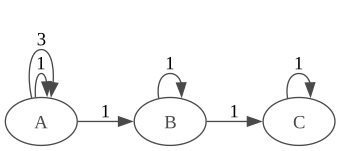
Fixing part of the LFSR’s seed and letting KTBNInference run past k=4 shows the kernel replicating – and the delayed relay through B and C:

kie = ktbn.KTBNInference(m)
kie.addObservation("A", 0, "1")
kie.addObservation("A", 2, "0")
kie.makeInference(10)  # horizon well beyond k=4: the kernel keeps replicating

for name in ["A", "B", "C"]:
  series = kie.posteriors(name)
  print(f"P({name}[t]=1 | A[0]=1, A[2]=0), t=0..{len(series) - 1} :")
  print([round(p.tolist()[1], 3) for p in series])

P(A[t]=1 | A[0]=1, A[2]=0), t=0..9 :
[1.0, 0.607, 0.0, 0.95, 0.413, 0.422, 0.578, 0.828, 0.57, 0.172]
P(B[t]=1 | A[0]=1, A[2]=0), t=0..9 :
[0.5, 0.5, 0.5, 0.4, 0.644, 0.501, 0.477, 0.565, 0.527, 0.534]
P(C[t]=1 | A[0]=1, A[2]=0), t=0..9 :
[0.5, 0.5, 0.5, 0.5, 0.444, 0.567, 0.494, 0.488, 0.528, 0.527]

gnb.plotFollowKTBN(m, ["A", "B", "C"], T=51, observations={"A[10]": 1, "A[11]": 1, "A[12]": 1})
gnb.plotFollowKTBN(m, ["A", "B", "C"], T=51, interventions={"A[10]": 1, "A[11]": 1, "A[12]": 1})

KTBNDatabaseGenerator draws trajectories from this fixed-CPT model, and KTBNLearner tries to recover a k-TBN back from them when k=4 is given (the true order). Structure learning from a finite sample does not always land on the exact causal direction, though: greedy hill climbing can settle for a statistically-equivalent but non-causal proxy – here, attributing A’s dependency to B (which is itself driven by A with a lag, and thus correlated with it) instead of to A directly. Compare the arcs and lags in learned.summaryGraph() below with the original one above:

gum.initRandom(42)  # reproducible sampling

dbgen = ktbn.KTBNDatabaseGenerator(m)
outdir = tempfile.mkdtemp()
dbgen.drawSamples(300, 60, outdir, "abc")  # 300 trajectories of length 60

schema = gum.BayesNet()
for name in list(m.temporalVarNames()) + list(m.atemporalVarNames()):
  schema.add(gum.LabelizedVariable(name, "", ["0", "1"]))

learner = ktbn.KTBNLearner(outdir, "abc", 300, 4, schema, m.atemporalVarNames())
learner.useScoreBIC().useGreedyHillClimbing()
learned = learner.learnKTBN()
gnb.sideBySide(learned, gnb.getDot(learned.summaryGraph()))

When k itself is unknown, KTBNAdaptiveLearner searches [2, kMax] and keeps the best-scoring order. Giving the search one extra slice of room removes the ambiguity above: a k=5 window lets the algorithm tell A’s own dual-lag dependency apart from its correlated echo in B, which shows up as a markedly better score for that candidate – exactly the kind of trade-off scorePerCandidateK() is meant to expose:

adaptive = ktbn.KTBNAdaptiveLearner(outdir, "abc", 300, 6, schema, m.atemporalVarNames())
adaptive.useScoreBIC().useGreedyHillClimbing()
best = adaptive.learnKTBN()
print("selected k :", adaptive.bestK())
print("score per candidate k :", adaptive.scorePerCandidateK())
gnb.sideBySide(best, gnb.getDot(best.summaryGraph()))

selected k : 5
score per candidate k : ((2, -43315.53041081031), (3, -43061.853978920604), (4, -42748.93405594639), (5, -30708.27259900556), (6, -35446.83614858938))

Markov chain : observation versus intervention

bn = gum.fastBN("A0{On|Off}->A1{On|Off}")
bn.cpt("A0").fillWith([1, 0])
bn.cpt("A1").fillWith([0.9, 0.1, 0, 1])
process = gum.KTBN.fromBN(bn)
gnb.sideBySide(
  process,
  gnb.getDot(process.summaryGraph()),
  gnb.getFollowKTBN(
    process,
    ["A"],
    T=51,
  ),
  captions=["Markov chain", "Its summary graph", "its behaviour"],
)

Markov chain

Its summary graph

its behaviour

gnb.flow.row(
  gnb.getFollowKTBN(process, ["A"], T=51, observations={"A[15]": "On"}),
  gnb.getFollowKTBN(process, ["A"], T=51, interventions={"A[15]": "On"}),
  captions=["With observation : if 'on' at t=15, then 'on' before", "With intervention : predictive maintenance"],
)

With observation : if 'on' at t=15, then 'on' before

With intervention : predictive maintenance