Using Continuous-Time Bayesian Networks

import pyagrum as gum
import pyagrum.lib.notebook as gnb
import pyagrum.ctbn as ct
import pyagrum.ctbn.notebook as ctbnnb

A CTBN(Continuous-Time Bayesian Networks) is a graphical model that allows a Bayesian Network to evolve over continuous time.

(For more details see https://pyagrum.readthedocs.io/en/latest/ctbn.html)

Creating a CTBN

# 1. Creating the ctbn
ctbn = ct.CTBN()

# 2. Adding the random variables
ctbn.add(gum.LabelizedVariable("cloudy?", "cloudy?"))
ctbn.add(gum.LabelizedVariable("rain?", "rain?"))

# 3. Adding the arcs
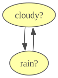
ctbn.addArc("cloudy?", "rain?")
ctbn.addArc("rain?", "cloudy?")

# 4. Filling the CIMS (Conditional Intensity Matrixes)
ctbn.CIM("cloudy?")[{"rain?": "0"}] = [[-0.1, 0.1], [1, -1]]
ctbn.CIM("cloudy?")[{"rain?": "1"}] = [[-100, 100], [0.5, -0.5]]

ctbn.CIM("rain?")[{"cloudy?": "0"}] = [[-0.5, 0.5], [1000, -1000]]
ctbn.CIM("rain?")[{"cloudy?": "1"}] = [[-2, 2], [2, -2]]

# 5. Plotting the CTBN (whith/whithout the CIMs)
ctbnnb.showCtbnGraph(ctbn)
ctbnnb.showCIMs(ctbn)

		cloudy?#j
rain?	cloudy?#i	0	1
0	0	-0.1000	0.1000
	1	1.0000	-1.0000
1	0	-100.0000	100.0000
	1	0.5000	-0.5000

CIM(cloudy?)

		rain?#j
cloudy?	rain?#i	0	1
0	0	-0.5000	0.5000
	1	1000.0000	-1000.0000
1	0	-2.0000	2.0000
	1	2.0000	-2.0000

CIM(rain?)

cloudy?#i gives the state cloudy? is currently in and cloudy?#j gives its next state.

The CIM object, built around a pyagrum.Tensor is used to store the parameters of the variables, describing the waiting time before switching to another state.

A useful tool for CIMs, mainly used for simple inference, is amalgamation. It allows to merge many CIMs into one.

cimA = ctbn.CIM("cloudy?")
cimB = ctbn.CIM("rain?")
amal = cimA.amalgamate(cimB)  # or cimA * cimB

amal.getTensor()  # as a Tensor

			cloudy?#i
rain?#i	cloudy?#j	rain?#j	0	1
0	0	0	-0.6000	1.0000
		1	0.5000	0.0000
	1	0	0.1000	-3.0000
		1	0.0000	2.0000
1	0	0	1000.0000	0.0000
		1	-1100.0000	0.5000
	1	0	0.0000	2.0000
		1	100.0000	-2.5000

print("\nJoint intensity matrix as numpy array\n")
print(amal.toMatrix())  # as a numpy array

Joint intensity matrix as numpy array

[[-6.0e-01  1.0e-01  5.0e-01  0.0e+00]
 [ 1.0e+00 -3.0e+00  0.0e+00  2.0e+00]
 [ 1.0e+03  0.0e+00 -1.1e+03  1.0e+02]
 [ 0.0e+00  2.0e+00  5.0e-01 -2.5e+00]]

A random variable of a ctbn can be identified by either its name or id.

In any case, most class functions parameters allow for a variable to be identified by either its name or id (type NameOrId).

labels_with_id = ctbn.labels(0)
labels_with_name = ctbn.labels("cloudy?")
print(f"labels using id : {labels_with_id}, using name : {labels_with_name}")

variable_with_id = ctbn.variable(0)
variable_with_name = ctbn.variable("cloudy?")
print(f"The variables 0 and 'cloudy?' are the same ? {variable_with_id == variable_with_name}")

labels using id : ('0', '1'), using name : ('0', '1')
The variables 0 and 'cloudy?' are the same ? True

All functions with NameOrId parameters work the same way

Random CTBN generator

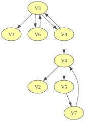
The CtbnGenerator module can be used to quickly generate CTBNs. The parameters value are drawn at random from a value range. The diagonal coefficients are just the negative sum of the ones on the same line (in a CIM). It is also possible to choose the number of variables, the maximum number of parents a variable can have, and the domain size of the variables.

randomCtbn = ct.randomCTBN(valueRange=(1, 10), n=8, parMax=2, modal=2)

ctbnnb.showCtbnGraph(randomCtbn)
ctbnnb.showCIMs(randomCtbn)

		V1#j
V3	V1#i	v1_1	v1_2
v3_1	v1_1	-3.5579	3.5579
	v1_2	5.9336	-5.9336
v3_2	v1_1	-6.9928	6.9928
	v1_2	8.7978	-8.7978

CIM(V1)

		V2#j
V4	V2#i	v2_1	v2_2
v4_1	v2_1	-4.6999	4.6999
	v2_2	5.4830	-5.4830
v4_2	v2_1	-8.0451	8.0451
	v2_2	9.8087	-9.8087

CIM(V2)

			V3#j
V6	V8	V3#i	v3_1	v3_2
v6_1	v8_1	v3_1	-3.9157	3.9157
		v3_2	2.2255	-2.2255
	v8_2	v3_1	-9.9001	9.9001
		v3_2	9.8740	-9.8740
v6_2	v8_1	v3_1	-3.7494	3.7494
		v3_2	5.5301	-5.5301
	v8_2	v3_1	-7.7686	7.7686
		v3_2	2.5621	-2.5621

CIM(V3)

			V4#j
V7	V8	V4#i	v4_1	v4_2
v7_1	v8_1	v4_1	-3.4758	3.4758
		v4_2	2.8830	-2.8830
	v8_2	v4_1	-2.7280	2.7280
		v4_2	1.4028	-1.4028
v7_2	v8_1	v4_1	-9.2305	9.2305
		v4_2	5.8492	-5.8492
	v8_2	v4_1	-9.6393	9.6393
		v4_2	5.3296	-5.3296

CIM(V4)

		V5#j
V4	V5#i	v5_1	v5_2
v4_1	v5_1	-9.3101	9.3101
	v5_2	5.4138	-5.4138
v4_2	v5_1	-9.3634	9.3634
	v5_2	1.4339	-1.4339

CIM(V5)

		V6#j
V3	V6#i	v6_1	v6_2
v3_1	v6_1	-6.6944	6.6944
	v6_2	2.8921	-2.8921
v3_2	v6_1	-6.2879	6.2879
	v6_2	8.6079	-8.6079

CIM(V6)

		V7#j
V5	V7#i	v7_1	v7_2
v5_1	v7_1	-2.2070	2.2070
	v7_2	2.3675	-2.3675
v5_2	v7_1	-7.5330	7.5330
	v7_2	7.5039	-7.5039

CIM(V7)

		V8#j
V3	V8#i	v8_1	v8_2
v3_1	v8_1	-8.5557	8.5557
	v8_2	3.1335	-3.1335
v3_2	v8_1	-4.5604	4.5604
	v8_2	5.3605	-5.3605

CIM(V8)

Inference with CTBNs

Exact inference & Forward Sampling inference

• Amalgamation is used to compute exact inference. It consists in merging all the CIMs of a CTBN into one CIM. Then we use the properties of markov process : \(P(X_t) = P(X_0)*exp(Q_Xt)\) for enough time to notice convergence.

• Forward sampling works this way:

  • At time \(t\) :

  • Draw a “time until next change” \(dt\) value for each variable’s exponential distribution of their waiting time.

  • Select the variable with smallest transition time : \(next time = t + dt\).

  • Draw the variable next state uniformly.

  • loop until \(t = timeHorizon\).

When doing forward sampling, we first iterate this process over a given amount of iterations (called burnIn). We consider the last values as the initial configuration for sampling. The reason is that the initial state of a CTBN is unknown without real data.

# 1. Initialiaze Inference object
ie = ct.SimpleInference(ctbn)
ie_forward = ct.ForwardSamplingInference(ctbn)
gnb.sideBySide(ctbnnb.getCtbnGraph(ctbn), ctbnnb.getCtbnInference(ctbn, ie), ctbnnb.getCtbnInference(ctbn, ie_forward))

In any case, inference can be made using makeInference() function from every Inference object.

import time

# Simple inference
time1 = time.time()
ie.makeInference(t=5000)
pot1 = ie.posterior("cloudy?")
elapsed1 = time.time() - time1

# Sampling inference
time2 = time.time()
ie_forward.makeInference(timeHorizon=5000, burnIn=100)
pot2 = ie_forward.posterior("cloudy?")
elapsed2 = time.time() - time2

gnb.sideBySide(
  gnb.getTensor(pot1),
  gnb.getTensor(pot2),
  captions=[f"Simple inference {round(elapsed1 * 1000, 2)} ms", f"Sampling inference {round(elapsed2 * 1000, 2)} ms"],
)

cloudy? 0 1 0.8334 0.1666 Simple inference 0.97 ms

cloudy? 0 1 0.8277 0.1723 Sampling inference 288.34 ms

Plotting a sample

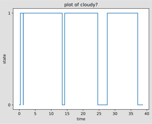
Here is an example of a trajectory plot

# 1_1. Find trajectory stored in the inference class
ie_forward.makeInference()
traj = ie_forward.trajectory  # a single trajectory list[tuple[float, str, str]]

# 1_2. Or find it in a csv file
ie_forward.writeTrajectoryCSV("out/trajectory.csv", n=1, timeHorizon=1000, burnIn=100)  # to save a trajectory
traj = ct.readTrajectoryCSV("out/trajectory.csv")  # a dict of trajectories

# 2. Plot the trajectory
ct.plotTrajectory(ctbn.variable("cloudy?"), traj[0], timeHorizon=40, plotname="plot of cloudy?")

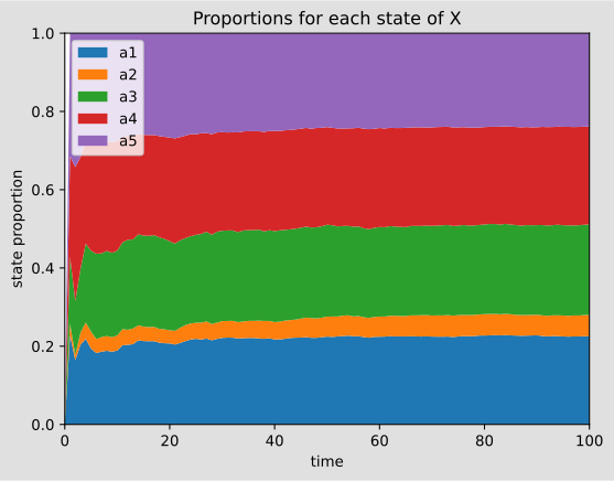
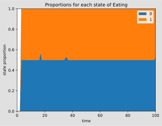
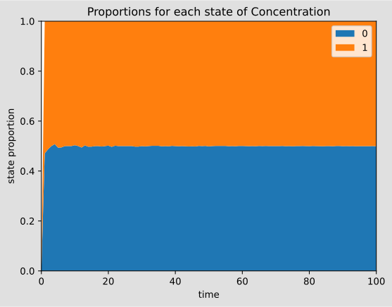
It is also possible to plot the proportions of the states a variable is in over time.

Let’s take the exemple of a variable with domain size=5.

# 1. Create CTBN
new_ctbn = ct.CTBN()
X = gum.LabelizedVariable("X", "X", ["a1", "a2", "a3", "a4", "a5"])
new_ctbn.add(X)
new_ctbn.CIM("X")[:] = [
  [-10, 2, 4, 0, 4],
  [0.5, -1, 0.5, 0, 0],
  [5, 0.5, -10, 3.5, 1],
  [50, 0.5, 50, -200.5, 100],
  [1, 0, 2, 7, -10],
]
# 2. Sampling
ieX = ct.ForwardSamplingInference(new_ctbn)
ieX.writeTrajectoryCSV("out/traj_quinary.csv", n=3, timeHorizon=100)
trajX = ct.readTrajectoryCSV("out/traj_quinary.csv")

# 3. Plotting
ct.plotFollowVar(X, trajX)

CTBN Learning with pyAgrum

The ctbn library has tools to learn the graph of a CTBN as well as the CIMs of its variables

Learning the variables

From a sample, we can find the variables name and their labels. However, if the sample is too short, it is possible that some information may be missed.

newCtbn = ct.CTBNFromData(traj)

print("variables found and their labels")
for name in newCtbn.names():
  print(f"variable {name}, labels : {newCtbn.labels(name)}")

variables found and their labels
variable cloudy?, labels : ('0', '1')
variable rain?, labels : ('0', '1')

Learning the structure of the CTBN

# 1. Create a Learner.
learner = ct.Learner("out/trajectory.csv")

# 2. Run learning algorithm
learned_ctbn = learner.learnCTBN()

# 3. Plot the learned CTBN
gnb.show(learned_ctbn)

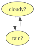
Let’s note that having a test object is necessary since we want to be able to test independency between variables. For now only 2 tests are available : (Fisher and Chi2) test and Oracle test. Oracle test is only used for benchmarking since it uses the initial ctbn as a reference.

Fitting parameters

It is also possible to approximate the transition time distributions of each variable, i.e the CIMs.

Note that conditioning variables are taken from the ctbn.

cims_before = ctbnnb.getCIMs(ctbn)
learner.fitParameters(ctbn)
cims_after = ctbnnb.getCIMs(ctbn)

gnb.sideBySide(cims_before, cims_after, captions=["original CIMs", "learned CIMs"])

cloudy?#j rain? cloudy?#i 0 1 0 0 -0.1000 0.1000 1 1.0000 -1.0000 1 0 -100.0000 100.0000 1 0.5000 -0.5000 CIM(cloudy?) rain?#j cloudy? rain?#i 0 1 0 0 -0.5000 0.5000 1 1000.0000 -1000.0000 1 0 -2.0000 2.0000 1 2.0000 -2.0000 CIM(rain?) original CIMs

cloudy?#j rain? cloudy?#i 0 1 0 0 -0.0880 0.0880 1 0.9920 -0.9920 1 0 -98.1810 98.1810 1 0.5060 -0.5060 CIM(cloudy?) rain?#j cloudy? rain?#i 0 1 0 0 -0.4870 0.4870 1 901.4790 -901.4790 1 0 -1.7550 1.7550 1 2.0800 -2.0800 CIM(rain?) learned CIMs

Example from [Nodelman et al, 2003]

This example comes from :

U. Nodelman, C.R. Shelton, and D. Koller (2003). "Learning Continuous Time Bayesian Networks." Proc. Nineteenth Conference on Uncertainty in Artificial Intelligence (UAI) (pp. 451-458).

# 1. Creating the ctbn
drugEffect = ct.CTBN()

drugEffect.add(gum.LabelizedVariable("Eating", ""))
drugEffect.add(gum.LabelizedVariable("Hungry", ""))
drugEffect.add(gum.LabelizedVariable("Full stomach", ""))
drugEffect.add(gum.LabelizedVariable("Uptake", ""))
drugEffect.add(gum.LabelizedVariable("Concentration", "?"))
drugEffect.add(gum.LabelizedVariable("Barometer", ""))
drugEffect.add(gum.LabelizedVariable("Joint pain", ""))
drugEffect.add(gum.LabelizedVariable("Drowsy", ""))

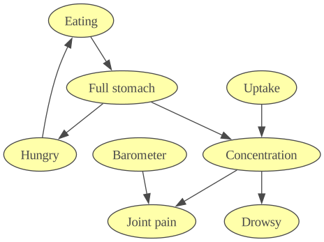
drugEffect.addArc("Hungry", "Eating")
drugEffect.addArc("Eating", "Full stomach")
drugEffect.addArc("Full stomach", "Hungry")
drugEffect.addArc("Full stomach", "Concentration")
drugEffect.addArc("Uptake", "Concentration")
drugEffect.addArc("Concentration", "Drowsy")
drugEffect.addArc("Barometer", "Joint pain")
drugEffect.addArc("Concentration", "Joint pain")

gnb.show(drugEffect)

from pyagrum.ctbn.CTBNGenerator import randomCIMs

randomCIMs(drugEffect, (0.1, 10))
drugEffect.CIM("Eating")[{"Hungry": 0}] = [[-0.1, 0.1], [10, -10]]
drugEffect.CIM("Eating")[{"Hungry": 1}] = [[-2, 2], [0.1, -0.1]]
drugEffect.CIM("Full stomach")[{"Eating": 0}] = [[-0.1, 0.1], [10, -10]]
drugEffect.CIM("Full stomach")[{"Eating": 1}] = [[-2, 2], [0.1, -0.1]]
drugEffect.CIM("Hungry")[{"Full stomach": 0}] = [[-0.1, 0.1], [10, -10]]
drugEffect.CIM("Hungry")[{"Full stomach": 1}] = [[-2, 2], [0.1, -0.1]]

ieX = ct.ForwardSamplingInference(drugEffect)
ieX.writeTrajectoryCSV("out/drugEffect.csv", n=3, timeHorizon=100)
trajX = ct.readTrajectoryCSV("out/drugEffect.csv")

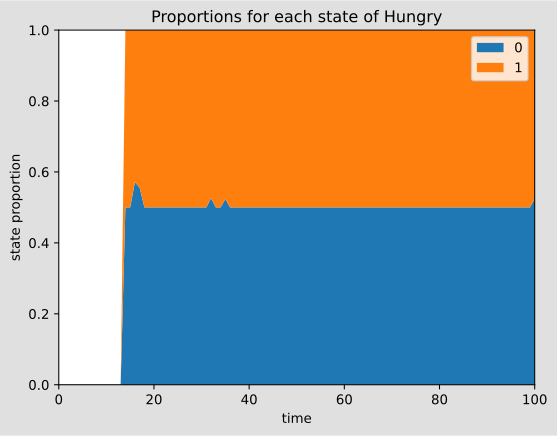
ct.plotFollowVar(drugEffect.variable("Hungry"), trajX)
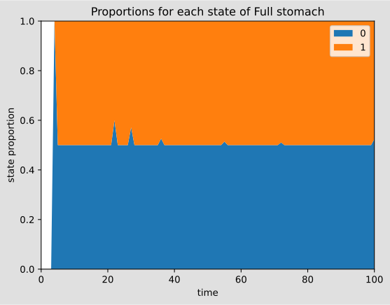
ct.plotFollowVar(drugEffect.variable("Full stomach"), trajX)
ct.plotFollowVar(drugEffect.variable("Eating"), trajX)
ct.plotFollowVar(drugEffect.variable("Concentration"), trajX)

Input/output with pickle for CTBN

import pickle

with open("out/testCTBN.pkl", "bw") as f:
  pickle.dump(drugEffect, f)
drugEffect

with open("out/testCTBN.pkl", "br") as f:
  copyDrug = pickle.load(f)
copyDrug